Buja et al. (2009) provides an inferential framework to assess whether residual plots indeed contain visual patterns inconsistent with the model assumptions. However, unlike conventional statistical tests that can be performed computationally in statistical software, the lineup protocol requires human evaluation of images. This characteristic makes it less suitable for large-scale applications, given the associated high labour costs and time requirements.
The autovi package aims to offer tools for automated
visual inference of residual plots. Currently, it only supports
diagnostic checks for classical normal linear regression models (CNLRM),
as the underlying computer vision models are specifically trained for
this model class. However, the autovi API is designed to be
extensible to other model types. This means you can obtain predictions
as long as you provide an appropriate method for generating null
residuals through the null_method argument.
Install the released version from CRAN with
install.packages("autovi")Install the development version from GitHub with:
# install.packages("remotes")
remotes::install_github("TengMCing/autovi")library(tidyverse)
library(autovi)All the available trained Keras models are listed in
list_keras_model(). All the trained Keras models listed
below will predict a visual signal strength for the visual patterns of
the input residual plot. This visual signal strength is essentially an
approximation of a Kullback–Leibler divergence based distance metric
which quantifies the difference between the actual residual distribution
and the reference residual distribution assumed under correct model
specification. Details about the methodologies are provided in our draft
paper https://github.com/TengMCing/auto_residual_reading/blob/master/paper/paper.pdf.
list_keras_model() %>% pull(model_name)
#> [1] "vss_32"      "vss_64"      "vss_128"     "vss_phn_32"  "vss_phn_64"
#> [6] "vss_phn_128"
Different Keras models are trained with residual plots obtained from different linear regression models violating various model assumptions.
vss_32, vss_64 and vss_128 are
trained with residual plots containing visual patterns indicating
non-linearity and heteroskedasticity issues. The number in the model
name represents the size of the input image. For instance,
32 means the input image has \(32
\times 32\) pixels.
vss_phn_32, vss_phn_64 and
vss_phn_128 are also trained with residual plots containing
visual patterns indicating non-linearity and heteroskedasticity, but the
visual patterns are more complex. Additionally, residual plots with
visual patterns of non-normality are also used for these models.
For this example, we will be using the vss_phn_32 Keras
model. The model can be obtained by using
get_keras_model().
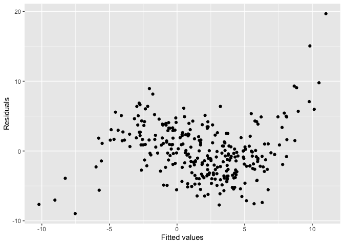
keras_model <- get_keras_model("vss_phn_32")To illustrate the use of this package, we will define an incorrectly specified model omitting certain higher-order terms of \(x\).
set.seed(2024)
x <- rnorm(300)
y <- 1 + x + x^2 + x^3 + rnorm(300, sd = 3)
this_model <- lm(y ~ x)
The residual plot of the fitted model shows a “S” shape indicating a non-linearity issue.
ggplot() +
  geom_point(aes(this_model$fitted.values, this_model$residuals)) +
  xlab("Fitted values") +
  ylab("Residuals")
To run diagnostics for this fitted model, we can initialize the
checker using auto_vi() and have a look at the input
residual plot using the plot_resid() method.
checker <- auto_vi(fitted_model = this_model, keras_model = keras_model)
checker$plot_resid()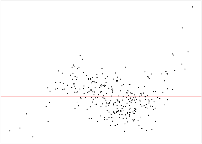
To predict the visual signal strength of this residual plot, simply
use the vss() method.
checker$vss()
#> ✔ Predict visual signal strength for 1 image.
#> # A tibble: 1 × 1
#>     vss
#>   <dbl>
#> 1  4.46
Having the visual signal strength of the residual plot is usually insufficient to determine if the model is correctly specified. Thus, we need to evaluate some null residual plots for comparison.
The checker includes a default method to generate null residuals
consistent with the null hypothesis that the fitted model is correctly
specified, which is the rotate_resid() method implementing
the residual rotation technique. This method is only suitable for
CNLRM.
checker$rotate_resid() %>%
  checker$plot_resid()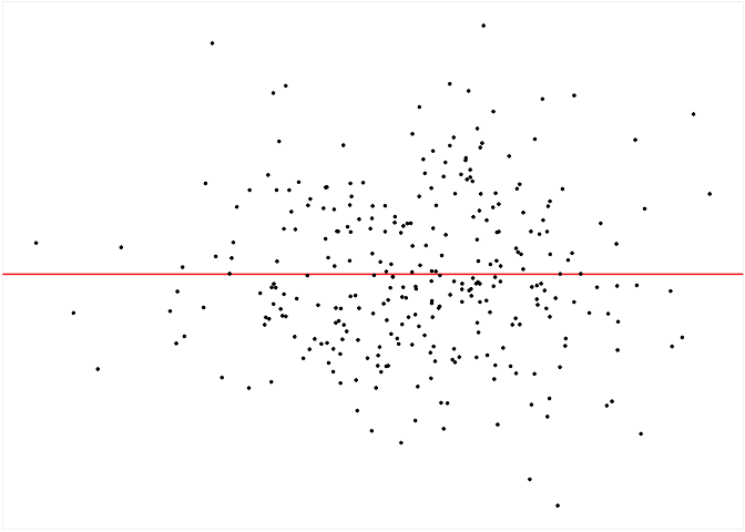
To get predictions for null residual plots, one can use the
null_vss() method. The keep_null_data and
keep_null_plot tells the method whether to preserve the
null residuals and null residuals plots in the result. For models that
needs to use a null generating method other than
rotate_resid(), the function can be provided via the
null_method argument. The only parameter of the provided
function should be fitted_model, which is the fitted model
object. And it should return a data frame with two columns
.fitted and .resid which are fitted values and
null residuals respectively.
checker$null_vss(20L,
                 keep_null_data = FALSE,
                 keep_null_plot = FALSE)
#> ✔ Generate null data.
#> ✔ Generate null plots.
#> ✔ Compute auxilary inputs.
#> ✔ Predict visual signal strength for 20 images.
#> # A tibble: 20 × 1
#>      vss
#>    <dbl>
#>  1 1.17
#>  2 1.09
#>  3 1.17
#>  4 0.773
#>  5 1.24
#>  6 0.640
#>  7 0.873
#>  8 1.06
#>  9 1.00
#> 10 1.01
#> 11 3.03
#> 12 1.15
#> 13 1.08
#> 14 0.910
#> 15 1.10
#> 16 0.913
#> 17 0.848
#> 18 1.08
#> 19 0.911
#> 20 0.665
If we want to measure the variation of the visual signal strength of
the residual plot, we can use the boot_vss() method to get
bootstrapped visual signal strength. This method resamples the
observations with replacement and refit the regression model. Similarly,
keep_boot_data and keep_boot_plot tells the
method whether to preserve bootstrapped residuals and plots.
checker$boot_vss(20L,
                 keep_boot_data = FALSE,
                 keep_boot_plot = FALSE)
#> ✔ Generate bootstrapped data.
#> ✔ Generate bootstrapped plots.
#> ✔ Compute auxilary inputs.
#> ✔ Predict visual signal strength for 20 images.
#> # A tibble: 20 × 1
#>      vss
#>    <dbl>
#>  1  4.20
#>  2  4.68
#>  3  5.56
#>  4  4.15
#>  5  4.37
#>  6  5.28
#>  7  4.36
#>  8  4.12
#>  9  4.70
#> 10  4.03
#> 11  4.11
#> 12  4.16
#> 13  5.09
#> 14  4.54
#> 15  3.83
#> 16  4.31
#> 17  4.72
#> 18  5.33
#> 19  4.85
#> 20  4.08
To run a comprehensive check including the analysis of null residuals
and bootstrapped residuals, use the check() method.
checker$check(null_draws = 20L, boot_draws = 20L)
#> ✔ Generate null data.
#> ✔ Generate null plots.
#> ✔ Compute auxilary inputs.
#> ✔ Predict visual signal strength for 20 images.
#> ✔ Generate bootstrapped data.
#> ✔ Generate bootstrapped plots.
#> ✔ Compute auxilary inputs.
#> ✔ Predict visual signal strength for 20 images.
#> ✔ Predict visual signal strength for 1 image.
The check result is stored in the check_result
attribute. If you print the checker object, it will show a
brief summary of the result.
checker
#>
#> ── <AUTO_VI object>
#> Status:
#>  - Fitted model: lm
#>  - Keras model: (None, 32, 32, 3) + (None, 5) -> (None, 1)
#>     - Output node index: 1
#>  - Result:
#>     - Observed visual signal strength: 4.461 (p-value = 0)
#>     - Null visual signal strength: [20 draws]
#>        - Mean: 1.14
#>        - Quantiles:
#>           ╔═════════════════════════════════════════════════╗
#>           ║   25%    50%    75%    80%    90%    95%    99% ║
#>           ║0.8896 1.0072 1.1204 1.2076 1.3012 1.5755 3.3615 ║
#>           ╚═════════════════════════════════════════════════╝
#>     - Bootstrapped visual signal strength: [20 draws]
#>        - Mean: 4.445 (p-value = 0)
#>        - Quantiles:
#>           ╔══════════════════════════════════════════╗
#>           ║  25%   50%   75%   80%   90%   95%   99% ║
#>           ║4.162 4.395 4.789 4.905 5.185 5.292 5.293 ║
#>           ╚══════════════════════════════════════════╝
#>     - Likelihood ratio: 0.7295 (boot) / 5.232e-14 (null) = 1.394e+13
A summary plot can be drawn with the summary_plot()
method. The solid line is the 95% sample quantile of the visual signal
strength predicted for null residual plots. The dot line is the visual
signal strength predicted for the original residual plot. The blue
density curve indicates the distribution of visual signal strength
predicted for null residual plots. And the red density curve indicates
the distribution of visual signal strength predicted for bootstrapped
residual plots.
The \(p\)-value is obtained by computing the ratio of null visual signal strength greater than or equal to observed visual signal strength. The red area along with the solid line indicates how often the fitted model would be considered incorrectly specified if the data can be repetitively drawn from the same data generating process.
For this example, the \(H_0\) is rejected because of small \(p\)-value. It can also be observed that almost all the time the refitted models will be considered as incorrectly specified, so this is a clear rejection. Furthermore, since two density curves are very different from each other, it is very unlikely the original residuals are from the same distribution of null residuals.
checker$summary_plot()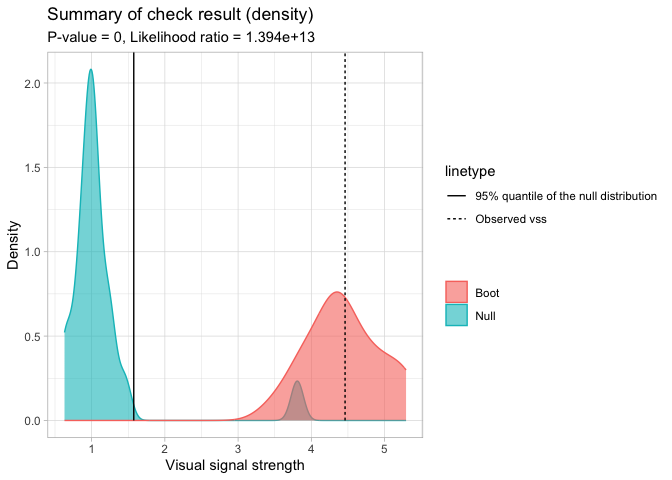
This package also enables the extraction of features from keras model
for other purposes. To extract features from a specific layer of the
keras model, one needs to provide the argument
extract_feature_from_layer. The following code chunk
extract features from the global pooling layer of the keras model.
checker$vss(extract_feature_from_layer = "global_max_pooling2d") %>%
  names()
#> ✔ Predict visual signal strength for 1 image.
#>   [1] "vss"   "f_1"   "f_2"   "f_3"   "f_4"   "f_5"   "f_6"   "f_7"   "f_8"
#>  [10] "f_9"   "f_10"  "f_11"  "f_12"  "f_13"  "f_14"  "f_15"  "f_16"  "f_17"
#>  [19] "f_18"  "f_19"  "f_20"  "f_21"  "f_22"  "f_23"  "f_24"  "f_25"  "f_26"
#>  [28] "f_27"  "f_28"  "f_29"  "f_30"  "f_31"  "f_32"  "f_33"  "f_34"  "f_35"
#>  [37] "f_36"  "f_37"  "f_38"  "f_39"  "f_40"  "f_41"  "f_42"  "f_43"  "f_44"
#>  [46] "f_45"  "f_46"  "f_47"  "f_48"  "f_49"  "f_50"  "f_51"  "f_52"  "f_53"
#>  [55] "f_54"  "f_55"  "f_56"  "f_57"  "f_58"  "f_59"  "f_60"  "f_61"  "f_62"
#>  [64] "f_63"  "f_64"  "f_65"  "f_66"  "f_67"  "f_68"  "f_69"  "f_70"  "f_71"
#>  [73] "f_72"  "f_73"  "f_74"  "f_75"  "f_76"  "f_77"  "f_78"  "f_79"  "f_80"
#>  [82] "f_81"  "f_82"  "f_83"  "f_84"  "f_85"  "f_86"  "f_87"  "f_88"  "f_89"
#>  [91] "f_90"  "f_91"  "f_92"  "f_93"  "f_94"  "f_95"  "f_96"  "f_97"  "f_98"
#> [100] "f_99"  "f_100" "f_101" "f_102" "f_103" "f_104" "f_105" "f_106" "f_107"
#> [109] "f_108" "f_109" "f_110" "f_111" "f_112" "f_113" "f_114" "f_115" "f_116"
#> [118] "f_117" "f_118" "f_119" "f_120" "f_121" "f_122" "f_123" "f_124" "f_125"
#> [127] "f_126" "f_127" "f_128" "f_129" "f_130" "f_131" "f_132" "f_133" "f_134"
#> [136] "f_135" "f_136" "f_137" "f_138" "f_139" "f_140" "f_141" "f_142" "f_143"
#> [145] "f_144" "f_145" "f_146" "f_147" "f_148" "f_149" "f_150" "f_151" "f_152"
#> [154] "f_153" "f_154" "f_155" "f_156" "f_157" "f_158" "f_159" "f_160" "f_161"
#> [163] "f_162" "f_163" "f_164" "f_165" "f_166" "f_167" "f_168" "f_169" "f_170"
#> [172] "f_171" "f_172" "f_173" "f_174" "f_175" "f_176" "f_177" "f_178" "f_179"
#> [181] "f_180" "f_181" "f_182" "f_183" "f_184" "f_185" "f_186" "f_187" "f_188"
#> [190] "f_189" "f_190" "f_191" "f_192" "f_193" "f_194" "f_195" "f_196" "f_197"
#> [199] "f_198" "f_199" "f_200" "f_201" "f_202" "f_203" "f_204" "f_205" "f_206"
#> [208] "f_207" "f_208" "f_209" "f_210" "f_211" "f_212" "f_213" "f_214" "f_215"
#> [217] "f_216" "f_217" "f_218" "f_219" "f_220" "f_221" "f_222" "f_223" "f_224"
#> [226] "f_225" "f_226" "f_227" "f_228" "f_229" "f_230" "f_231" "f_232" "f_233"
#> [235] "f_234" "f_235" "f_236" "f_237" "f_238" "f_239" "f_240" "f_241" "f_242"
#> [244] "f_243" "f_244" "f_245" "f_246" "f_247" "f_248" "f_249" "f_250" "f_251"
#> [253] "f_252" "f_253" "f_254" "f_255" "f_256"
To check all the available layer names, one can list them with the
KERAS_WRAPPER class.
KERAS_WRAPPER$list_layer_name(keras_model)
#>  [1] "input_1"                  "tf.__operators__.getitem"
#>  [3] "tf.nn.bias_add"           "grey_scale"
#>  [5] "block1_conv1"             "batch_normalization"
#>  [7] "activation"               "block1_conv2"
#>  [9] "batch_normalization_1"    "activation_1"
#> [11] "block1_pool"              "dropout"
#> [13] "block2_conv1"             "batch_normalization_2"
#> [15] "activation_2"             "block2_conv2"
#> [17] "batch_normalization_3"    "activation_3"
#> [19] "block2_pool"              "dropout_1"
#> [21] "block3_conv1"             "batch_normalization_4"
#> [23] "activation_4"             "block3_conv2"
#> [25] "batch_normalization_5"    "activation_5"
#> [27] "block3_conv3"             "batch_normalization_6"
#> [29] "activation_6"             "block3_pool"
#> [31] "dropout_2"                "block4_conv1"
#> [33] "batch_normalization_7"    "activation_7"
#> [35] "block4_conv2"             "batch_normalization_8"
#> [37] "activation_8"             "block4_conv3"
#> [39] "batch_normalization_9"    "activation_9"
#> [41] "block4_pool"              "dropout_3"
#> [43] "block5_conv1"             "batch_normalization_10"
#> [45] "activation_10"            "block5_conv2"
#> [47] "batch_normalization_11"   "activation_11"
#> [49] "block5_conv3"             "batch_normalization_12"
#> [51] "activation_12"            "block5_pool"
#> [53] "dropout_4"                "global_max_pooling2d"
#> [55] "additional_input"         "concatenate"
#> [57] "dense"                    "dropout_5"
#> [59] "activation_13"            "dense_1"
While running the comprehensive check with the check()
method, one can provide the extract_feature_from_layer
argument to extract features.
checker$check(null_draws = 20L, boot_draws = 20L, extract_feature_from_layer = "global_max_pooling2d")
#> ✔ Generate null data.
#> ✔ Generate null plots.
#> ✔ Compute auxilary inputs.
#> ✔ Predict visual signal strength for 20 images.
#> ✔ Generate bootstrapped data.
#> ✔ Generate bootstrapped plots.
#> ✔ Compute auxilary inputs.
#> ✔ Predict visual signal strength for 20 images.
#> ✔ Predict visual signal strength for 1 image.
The features are also stored in the check_result
attribute.
checker$check_result$observed
#> # A tibble: 1 × 257
#>     vss   f_1    f_2   f_3   f_4   f_5     f_6    f_7   f_8    f_9  f_10  f_11
#>   <dbl> <dbl>  <dbl> <dbl> <dbl> <dbl>   <dbl>  <dbl> <dbl>  <dbl> <dbl> <dbl>
#> 1  4.46 0.167 0.0687     0     0     0 0.00164 0.0695     0 0.0847     0     0
#> # ℹ 245 more variables: f_12 <dbl>, f_13 <dbl>, f_14 <dbl>, f_15 <dbl>,
#> #   f_16 <dbl>, f_17 <dbl>, f_18 <dbl>, f_19 <dbl>, f_20 <dbl>, f_21 <dbl>,
#> #   f_22 <dbl>, f_23 <dbl>, f_24 <dbl>, f_25 <dbl>, f_26 <dbl>, f_27 <dbl>,
#> #   f_28 <dbl>, f_29 <dbl>, f_30 <dbl>, f_31 <dbl>, f_32 <dbl>, f_33 <dbl>,
#> #   f_34 <dbl>, f_35 <dbl>, f_36 <dbl>, f_37 <dbl>, f_38 <dbl>, f_39 <dbl>,
#> #   f_40 <dbl>, f_41 <dbl>, f_42 <dbl>, f_43 <dbl>, f_44 <dbl>, f_45 <dbl>,
#> #   f_46 <dbl>, f_47 <dbl>, f_48 <dbl>, f_49 <dbl>, f_50 <dbl>, f_51 <dbl>, …
This package provide ways to conduct PCA on these features. The
feature_pca method will combine the features obtained from
the prediction of the observed residual plot, null residual plots, and
the bootstrapped residual plots, then conduct PCA on them. The results
are the rotated features. The variable set provides the set
label of the observation, which can either be “observed”, “null” or
“boot”.
checker$feature_pca()
#> # A tibble: 41 × 298
#>      f_1    f_2   f_3   f_4   f_5     f_6    f_7   f_8    f_9  f_10  f_11  f_12
#>    <dbl>  <dbl> <dbl> <dbl> <dbl>   <dbl>  <dbl> <dbl>  <dbl> <dbl> <dbl> <dbl>
#>  1 0.167 0.0687  0     0    0     0.00164 0.0695 0     0.0847 0     0     0.149
#>  2 1.08  4.14    4.10  5.43 2.35  2.04    3.09   2.39  2.01   1.94  4.32  2.43
#>  3 1.10  2.85    2.90  3.08 1.20  1.21    1.69   1.50  1.59   0.828 2.55  1.75
#>  4 0.827 3.20    2.92  3.45 1.50  1.28    1.89   1.61  1.64   1.28  2.66  1.71
#>  5 0.955 3.85    3.74  5.17 2.24  1.97    2.96   2.25  1.81   1.91  4.04  2.23
#>  6 1.22  3.60    3.70  4.70 2.00  1.72    2.66   2.19  1.77   1.57  3.83  2.18
#>  7 1.21  3.41    3.51  4.22 1.75  1.58    2.37   1.99  1.75   1.33  3.47  2.08
#>  8 1.09  3.00    3.04  3.71 1.53  1.40    2.12   1.76  1.53   1.16  3.01  1.85
#>  9 1.02  2.87    2.84  3.42 1.42  1.28    1.94   1.65  1.45   1.09  2.75  1.70
#> 10 0.570 1.72    1.25  1.36 0.270 0.342   0.419  0.545 0.959  0.267 0.913 0.875
#> # ℹ 31 more rows
#> # ℹ 286 more variables: f_13 <dbl>, f_14 <dbl>, f_15 <dbl>, f_16 <dbl>,
#> #   f_17 <dbl>, f_18 <dbl>, f_19 <dbl>, f_20 <dbl>, f_21 <dbl>, f_22 <dbl>,
#> #   f_23 <dbl>, f_24 <dbl>, f_25 <dbl>, f_26 <dbl>, f_27 <dbl>, f_28 <dbl>,
#> #   f_29 <dbl>, f_30 <dbl>, f_31 <dbl>, f_32 <dbl>, f_33 <dbl>, f_34 <dbl>,
#> #   f_35 <dbl>, f_36 <dbl>, f_37 <dbl>, f_38 <dbl>, f_39 <dbl>, f_40 <dbl>,
#> #   f_41 <dbl>, f_42 <dbl>, f_43 <dbl>, f_44 <dbl>, f_45 <dbl>, f_46 <dbl>, …